Part 1: Tokenization and embeddings

This chapter covers the first real step in the Transformer pipeline: turning text into token IDs and then turning those IDs into learned vectors. Tokenization is not a separate numbered chapter in this course; it is the front end of the embedding story. The math bridge explains the one-hot and matrix-product view behind the lookup.

Foundation connection: vector geometry defines length and cosine similarity, while backpropagation shows why an embedding row can learn from next-token loss. Here we apply both ideas to the concrete lookup table and context examples.

Start with the whole prediction path if embedding and output projection sound like disconnected steps. This chapter zooms in on where the first vector comes from and how a final vector becomes token scores.

1. What is a language model?

A language model is a probability distribution over sequences of tokens.

The basic goal is to model:

\[ P(w_1, w_2, \dots, w_n) \]

or more practically,

\[ P(w_t \mid w_1, w_2, \dots, w_{t-1}) \]

This says: given the previous text, how likely is the next token?

A language model is therefore a system that learns how to predict the next symbol in a sequence.

Example

Suppose the model sees:

“The cat sat on the …”

It might assign high probability to:

• mat
• chair
• floor

and lower probability to:

• banana
• airplane

The model is not just memorizing strings. It is learning statistical structure in language.

Why this matters

Language modeling is the foundation of:

• autocomplete
• translation
• summarization
• chatbots
• coding assistants
• retrieval and reasoning systems

The central question is always the same:

How do we represent text so that a machine can learn patterns in it?

1.5. Why the same token can mean different things in different contexts

A token embedding is a start, not the end of the story.

The same word can appear in multiple contexts with different meanings. Consider:

• “American shrew mole”
• “one mole of carbon dioxide”
• “take a biopsy of the mole”

The token “mole” is the same string, but the surrounding context changes its meaning. The initial embedding row for “mole” is the same in all three cases because it is just a lookup vector. It does not yet know the surrounding sentence.

This is the exact reason attention exists.

The model must transform that generic representation into a context-specific one by reading nearby tokens. In a good Transformer block, the representation of “mole” is adjusted so that it points in a direction appropriate for the local meaning: mammal, unit, or lesion.

The same pattern applies to “tower.” In one context it may be the Eiffel tower; in another it may be a radio tower; in another it may be a miniature tower in a toy city. The generic embedding of “tower” is broad. The surrounding words reshape it into a more precise semantic direction.

This is the central idea behind contextual embeddings: a word is not defined only by its own lexical row, but by the surrounding information it absorbs from the sequence.

A nice way to think about it is this:

• the initial token embedding encodes the word identity
• the attention block adds context-dependent updates
• the refined vector can move to a different region of embedding space depending on what is around it

This is why the representation geometry matters so much. We are not merely storing word IDs; we are learning a vector space where direction and neighborhood structure encode meaning.

2. The representation problem

A computer does not understand words directly. It understands numbers.

So before a model can predict the next token, it must first encode text into a numeric representation.

This is the key idea:

All of the following are forms of encoding:

• one-hot vectors
• count vectors
• TF-IDF vectors
• co-occurrence matrices
• SVD-based latent vectors
• neural word embeddings
• position-aware embeddings

They are all attempts to map symbols into a space where mathematical operations can be performed.

A conceptual framework

We can view language representation as a pipeline:

\[ \text{string} \rightarrow \text{token sequence} \rightarrow \text{encoding} \rightarrow \text{dense vector space} \rightarrow \text{model} \]

The main question is not “what is the final representation?” but:

What structure should the encoding preserve?

Should it preserve:

• token identity?
• document frequency?
• context similarity?
• semantic similarity?
• order?

Different methods solve different parts of this problem.

Diagram: the representation pipeline

3. What is a token?

A token is the unit of text that the model works with.

Examples:

• a whole word
• a subword piece
• a character
• a byte
• a learned symbol from a tokenizer

This is analogous to images being built from pixels and audio from samples.

The choice of tokenization matters because it changes the vocabulary and the geometry of the problem.

Examples:

• word-level: “unbelievable” is one token
• subword-level: “un”, “believ”, “able”
• character-level: “u”, “n”, “b”, “e” ...

No tokenization is universally best. It is a design tradeoff between:

• vocabulary size
• sequence length
• rare-word handling
• efficiency
• semantic precision

A token ID is an index into a learned table

Suppose the vocabulary has four tokens and the model width is two. Its embedding table might currently be

\[ E=\begin{bmatrix} 0.1&0.2\\ -0.4&0.3\\ 0.8&-0.1\\ 0.0&0.5 \end{bmatrix},\qquad E\in\mathbb R^{4\times2}. \]

Token ID 2 selects row 2 (counting from zero): \(E[2]=[0.8,-0.1]\). In one-hot notation \([0,0,1,0]E=[0.8,-0.1]\); software usually performs a direct row lookup rather than constructing the one-hot vector. For IDs [2,0,2], the output shape is \((3,2)\) and the first and third rows are initially identical because they select the same parameter row.

The table values usually start from an initialization, not a dictionary of human meanings. During language-model training, loss gradients flow backward through the Transformer to the rows used by the batch. If the accumulated gradient for row 2 is \([0.2,-0.4]\), one plain gradient-descent step with learning rate \(0.1\) gives \([0.8,-0.1]-0.1[0.2,-0.4]=[0.78,-0.06]\). If an ID occurs more than once, its contributions combine. Real training commonly uses AdamW rather than this one-step illustration.

Static lookup versus contextual representation

The embedding row for token ID 2 is the same wherever that ID appears. After attention and MLP layers, its hidden state can differ by context. For river bank and bank account, the tokenizer may produce the same ID for bank, so the initial row is the same; neighboring tokens and attention can produce different later states. Tokenization chooses the discrete pieces, the embedding table supplies trainable starting vectors, and the Transformer makes their representations context dependent.

This distinction is easy to lose when people call both the table row and a later hidden state an “embedding.” In this course, token embedding means the lookup vector; contextual representation means a state after sequence processing.

Trace the lookup back to the output

The input table and the output projection answer different questions. The input table asks, “Given an ID, which starting vector should I use?” The output projection asks, “Given a final state, what score should each possible next ID receive?” Using rows for token vectors, their shapes are:

Step	Calculation	Shape
Select ID \(i\)	\(x=E[i]\)	\(E:(V,d)\); \(x:(d,)\)
Add position and process context	\(h=\operatorname{Transformer}(x,\text{prefix})\)	\(h:(d,)\)
Score vocabulary	\(z=hU+b\)	\(U:(d,V)\); \(z:(V,)\)
Normalize	\(p=\operatorname{softmax}(z)\)	\(p:(V,)\)

For an intentionally small example, take \(h=[2,1]\) and let the three columns of \(U\) be \(u_0=[1,0]\), \(u_1=[0,1]\), and \(u_2=[1,1]\), with zero bias. The three logits are the dot products \([h\cdot u_0,h\cdot u_1,h\cdot u_2]=[2,1,3]\). Softmax gives approximately \([0.245,0.090,0.665]\). The largest probability belongs to ID 2. These columns are learned output weights; their dot products are scores, and softmax is what makes probabilities. The foundation softmax section shows why the exponentials and normalization are needed.

Some models tie the weights by setting \(U=E^\top\), so the same learned table participates at input and output. Others learn a separate \(U\). Weight tying shares parameters; it does not make the contextual state \(h\) equal to the starting row \(E[i]\). At training time, every eligible position has its own \(h_t\) and output distribution. At generation time, the newest position's distribution selects the continuation.

For a visual companion to this lookup-to-output path, see 3Blue1Brown's Transformer lesson. The teaching style is simplified for intuition, while this chapter keeps the token-to-lookup story concrete and original.

4. One-hot encoding: identity without meaning

The simplest representation is one-hot encoding.

If the vocabulary size is \(V\), each token is a vector of length \(V\) with a single 1 and zeros elsewhere.

Example:

\[ \text{cat} = [0, 1, 0, 0, \dots] \]

\[ \text{dog} = [0, 0, 1, 0, \dots] \]

This is mathematically valid, but it is semantically weak.

It tells the model:

• this is token 42
• this is token 77

It does not tell the model:

• cat is close to kitten
• dog is close to puppy
• king is close to queen

The issue is that all one-hot vectors are orthogonal.

So the representation sees every token as equally far from every other token.

Diagram: one-hot geometry

flowchart LR
    A[cat] --> B[one-hot vector]
    C[dog] --> B
    D[kitten] --> B
    B --> E[all vectors are equally distant]

This is the first serious problem: we want similarity structure, not just identity labels.

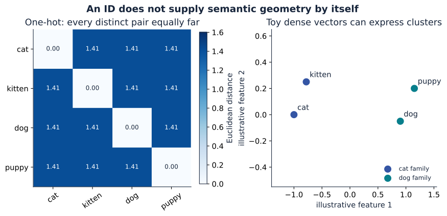
The right-hand points are chosen for illustration, not trained model embeddings. The plot shows what dense coordinates can express; the next sections explain how data and objectives can shape such coordinates. Regenerate this and the other course plots with python examples/plot_foundations.py from the repository root.

5. The geometry of meaning

A useful representation should encode semantic similarity.

We want a vector space where:

• cat is near kitten
• dog is near puppy
• doctor is near hospital
• France is near Paris

This is a geometric statement.

Two common similarity measures are:

• Euclidean distance
• cosine similarity

The cosine similarity is:

\[ \cos(\theta) = \frac{u \cdot v}{\|u\|\|v\|} \]

If two vectors point in nearly the same direction, their cosine similarity is large.

This is the foundation for embedding-based semantics: vectors are placed so that similar meanings are close in space.

Similarity is an empirical property to test, not a promise of the lookup operation. A token can have several senses, subword pieces need not correspond to whole words, and raw embedding neighbors can differ from neighbors after context processing. An analogy such as \(v_{\rm king}-v_{\rm man}+v_{\rm woman}\approx v_{\rm queen}\) can illustrate a direction in some trained spaces, but it is not a law of vector arithmetic or a reliable definition of meaning. The safer exercise is to compute nearest neighbors for a specified trained table, then inspect successes and failures.

Diagram: semantic clusters

flowchart LR
    A[cat] --> S[embedding space]
    B[kitten] --> S
    C[dog] --> S
    D[puppy] --> S
    E[car] --> S
    F[truck] --> S
    S --> G[related tokens cluster together]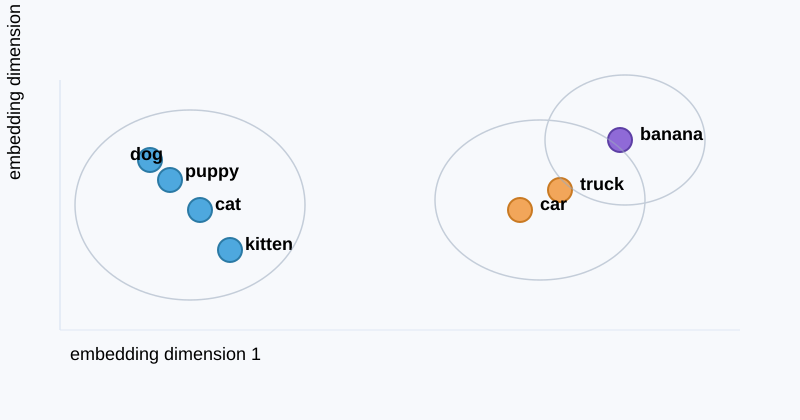

6. Count-based representations: statistics before learned semantics

The first real step beyond one-hot encoding used counts from corpora.

6.1 Document-term matrix

For a collection of documents, we can construct a matrix:

\[ X \in \mathbb{R}^{n \times V} \]

where \(X_{ij}\) is how often token \(j\) appears in document \(i\).

This gives a numeric representation for each document.

Example

Document	cat	dog	pet	car	drive
\(d_1\)	3	0	2	0	0
\(d_2\)	0	2	1	3	3

This is a count vector representation.

Why counts matter

Counts encode frequency. A word that appears often in a document is more important there.

But they also have major weaknesses:

• common words dominate
• order is lost
• context is weak
• repeated patterns do not necessarily reflect meaning

The bag-of-words model ignores sequence structure completely.

6.2 TF-IDF

TF-IDF improves on raw counts by balancing local and global importance.

\[ \mathrm{TFIDF}(t, d) = \mathrm{TF}(t, d) \cdot \mathrm{IDF}(t) \]

where:

• \(\mathrm{TF}(t,d)\) measures how often term \(t\) appears in document \(d\)
• \(\mathrm{IDF}(t)\) downweights very common words

This tells us the following:

• words that occur a lot in one document are important there
• words that appear everywhere are less informative

This was a big step, but still shallow compared with learned embeddings.

Diagram: count-to-statistical representation

flowchart TD
    A[Corpus] --> B[Word counts]
    B --> C[Document-term matrix]
    C --> D[Bag-of-words]
    D --> E[TF-IDF weighting]
    E --> F[Improved statistical representation]

7. Why SVD appears: compressing the token space

The next deep idea is latent structure.

A count matrix is large, sparse, and noisy. But often there are hidden patterns underneath it.

The main intuition is:

The data is not random. There are some low-dimensional semantic factors that explain much of it.

This is where SVD comes in.

First-principles view

Suppose we have a document-term matrix \(X\).

We want a lower-dimensional approximation:

\[ X \approx U_k \Sigma_k V_k^T \]

where:

• \(U_k\) captures document factors
• \(V_k\) captures token factors
• \(\Sigma_k\) gives the importance of each factor

This is not magic. It is the best low-rank approximation in the least-squares sense.

Why people tried SVD

Because the raw matrix is huge and redundant.

If two words tend to appear in similar documents, they are likely related semantically. We want to discover those hidden patterns and compress them.

So SVD is used to answer:

Can we represent the original token-document relationships in a smaller space without losing the important structure?

This is the first major step from raw counts to latent semantics.

A key example

Imagine a matrix where rows are documents and columns are words.

The word “bank” appears near contexts like:

• finance
• loan
• credit
• river
• shore
• water

A low-rank factorization may represent “bank” using latent components influenced by contexts such as:

• financial context
• geographic context

However, a basic count matrix still gives the token one vector; it does not choose a separate meaning for each occurrence. Contextual token states later in a Transformer can differ between river bank and bank account.

Why this is important

This is the bridge from:

• token counts
• to latent semantic dimensions
• to learned embeddings

It is one of the first times the model is encouraged to think of meaning as geometry.

Diagram: low-rank semantic compression

flowchart LR
    A[High-dimensional count matrix] --> B[Find dominant latent directions]
    B --> C[Low-rank approximation]
    C --> D[Semantic subspace]
    D --> E[Compact token representation]

SVD as a token-to-latent mapping

SVD can be interpreted as mapping each token into a lower-dimensional latent space.

For the document-by-token matrix \(X\in\mathbb R^{n\times V}\) used above, document coordinates come from rows of \(U_k\Sigma_k\), while token coordinates come from rows of \(V_k\Sigma_k\) (one common scaling convention). The row/column choice matters: \(U_k\) has one row per document, not one row per token.

So in a very real sense,

SVD converts a token from a sparse, high-dimensional symbol into a dense latent semantic vector.

This is the conceptual step that leads directly into word embeddings.

8. Word2Vec: learning meaning from context

The key conceptual jump is this:

Words are not defined only by their own identity. They are defined by the contexts in which they appear.

Figure 1 from Mikolov et al., Efficient Estimation of Word Representations in Vector Space (2013). CBOW predicts the center word from surrounding context; Skip-gram predicts surrounding words from the center word.

Context is supervision

In a sentence like:

“The doctor treated the patient at the hospital.”

The word “doctor” is related to “patient,” “hospital,” and “treated.”

This is not because of explicit labels. It is because those words frequently appear in similar local contexts.

Word2Vec learns exactly that.

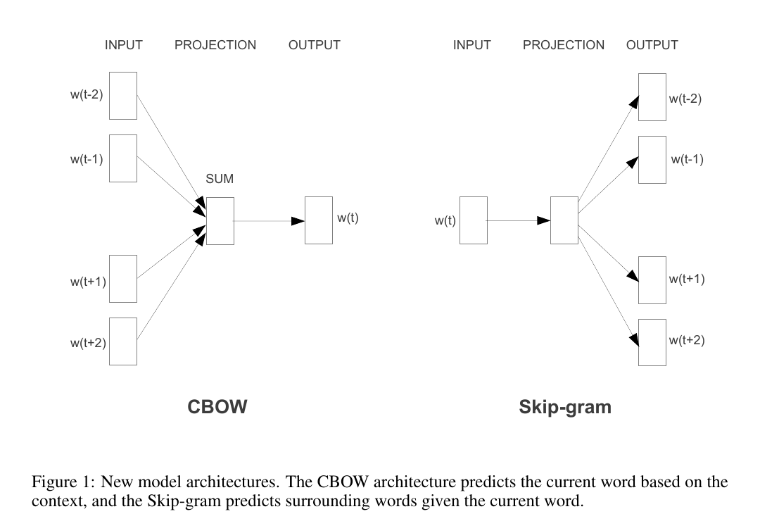
Skip-gram objective

Skip-gram tries to predict surrounding words from a center word.

For a center token \(w_t\) and context tokens \(w_{t-k}, ..., w_{t+k}\), it maximizes:

\[ P(w_{t+j} \mid w_t) \]

for nearby positions \(j\).

This encourages words that appear in similar contexts to have nearby vectors.

CBOW objective

CBOW does the opposite:

It predicts the center word from surrounding context words.

Both objectives move the embedding vectors so that contextually similar words become close together.

Why this is powerful

The word “bank” can appear in contexts involving:

• finance
• loans
• deposits
• rivers
• shore
• water

The model learns the meaning from context, not from a fixed dictionary entry.

So the embedding is not just a name. It is a compressed summary of usage patterns.

Diagram: context-based learning

flowchart LR
    A[center word: bank] --> B[observe context]
    B --> C[finance context]
    B --> D[river context]
    C --> E[embedding learns financial meaning]
    D --> F[embedding learns geographic meaning]
    E --> G[semantic geometry]
    F --> G

A small code example: context similarity

import numpy as np

# toy vectors representing word meaning in a learned embedding space
bank_finance = np.array([1.0, 0.9, 0.2])
loan = np.array([0.9, 1.0, 0.1])
river = np.array([0.2, 0.1, 1.0])
shore = np.array([0.1, 0.2, 0.9])


def cosine(a, b):
    return float(np.dot(a, b) / (np.linalg.norm(a) * np.linalg.norm(b)))

print("bank vs loan:", cosine(bank_finance, loan))
print("bank vs river:", cosine(bank_finance, river))

This shows the idea: words with similar roles in context occupy similar directions in vector space.

9. From embeddings to sequence models

Embeddings solve the token representation problem, but they do not yet solve order.

Consider:

• “the cat sat”
• “the sat cat”

The token set is the same, but the sentence is different.

The model must know not only what words exist, but where they are in time.

This is where sequence models enter the picture.

10. Why recurrent models appear in this story

An embedding table alone has no sequence memory. Recurrent neural networks introduced a state that updates as each token arrives. LSTMs added gates and a cell state to improve long-range learning. The optional LSTM appendix works through recurrence, vanishing gradients, three gates and a candidate update, and a two-step numerical example. It also shows how encoder-decoder attention bridged recurrent models and Transformers. Continue directly to Part 2 if your focus is the Transformer.

11. The full arc: from text to transformer

The correct historical story is:

1. language is symbolic and discrete
2. we need some encoding of text into numbers
3. one-hot encoding is too weak because it loses similarity
4. counts and TF-IDF add frequency structure
5. SVD reveals lower-dimensional latent semantics
6. Word2Vec learns semantic vectors from context
7. sequence models add order, but have bottlenecks
8. transformers replace recurrence with direct attention over context

The key theme is coherence:

The task is not to discover a single magical vector. It is to construct a representation that preserves meaning, context, and sequence structure.

12. The embedding layer inside a Transformer, mathematically

The earlier sections explain where embeddings came from. We can now state exactly how a Transformer uses and learns them.

12.1 The embedding table is a learned matrix

Let:

• \(V\) be the vocabulary size
• \(d\) be the model width
• \(T\) be the sequence length
• \(E\in\mathbb{R}^{V\times d}\) be the token embedding matrix
• \(x_t\in\{0,\ldots,V-1\}\) be the token ID at position \(t\)

The embedding layer performs a row lookup:

\[ e_t=E[x_t,:]\in\mathbb{R}^{d}. \]

The same operation can be written as matrix multiplication. If \(o(x_t)\in\mathbb{R}^{V}\) is the one-hot row vector for token \(x_t\), then

\[ e_t=o(x_t)E. \]

The one-hot vector contains no learned meaning. It merely selects a row. Implementations use an indexed lookup because constructing a length-\(V\) one-hot vector would waste memory and computation.

For a batch of token IDs \(X\in\{0,\ldots,V-1\}^{B\times T}\), the lookup returns

\[ E[X]\in\mathbb{R}^{B\times T\times d}. \]

Each of the \(BT\) token occurrences now has a \(d\)-dimensional starting vector. If the same ID occurs several times, every occurrence starts with the same row of \(E\).

12.2 What exactly is learned in the embedding layer?

The \(Vd\) numbers in \(E\) are trainable parameters. They usually begin as small random values. No coordinate is initially assigned a human label such as “animal,” “past tense,” or “formal language.” Training changes the rows so the entire network becomes better at its prediction objective.

What a row learns is therefore operational:

\(E[v,:]\) becomes a useful starting representation for token \(v\) because that representation helps the later Transformer layers reduce prediction loss across all contexts where \(v\) occurs.

Tokens used in similar predictive contexts often receive related gradient updates, which can create semantic and syntactic geometry. That geometry is learned from the task; the lookup operation itself does not guarantee it.

The individual axes are not uniquely meaningful. If the embedding space and the following learned matrices were rotated together, the network could represent the same function in a different coordinate basis. Distances, directions, and downstream behavior are usually more informative than trying to name coordinate 17.

Frequency also matters. A common token contributes to many training examples and its row is updated often. A rare token receives fewer direct input-side updates. Subword tokenization helps by letting rare words share reusable pieces.

12.3 Position turns a token row into a sequence input

A lookup answers which token is this? It does not answer where did it occur? With additive position encoding, the first layer receives

\[ h_t^{(0)}=\sqrt d\,E[x_t,:]+P_t, \]

where \(P_t\in\mathbb{R}^{d}\) is either a fixed sinusoidal vector or a row from a learned position table. The scale \(\sqrt d\) is the convention used in the original Transformer; architectures may vary.

For the sentence “the cat sat,” the model constructs

\[ H^{(0)}= \begin{bmatrix} \sqrt d\,E[x_{\text{the}}]+P_0\\ \sqrt d\,E[x_{\text{cat}}]+P_1\\ \sqrt d\,E[x_{\text{sat}}]+P_2 \end{bmatrix} \in\mathbb{R}^{3\times d}. \]

The token row supplies identity-related features; \(P_t\) supplies order. Part 2 derives fixed sinusoidal encoding, learned additive positions, and RoPE. With RoPE, a model normally does not add \(P_t\) here. It rotates query and key pairs later inside each attention layer.

12.4 Attention and the FFN create contextual states

The initial row for “bank” is static. It is the same lookup in “river bank” and “bank account.” Transformer blocks turn that static starting vector into a context-dependent hidden state.

Using a common pre-norm decoder block notation, layer \(\ell\) computes

\[ A^{(\ell)}=H^{(\ell-1)}+ \operatorname{MHA}\!\left(\operatorname{LN}(H^{(\ell-1)})\right), \]

\[ H^{(\ell)}=A^{(\ell)}+ \operatorname{FFN}\!\left(\operatorname{LN}(A^{(\ell)})\right). \]

These two sublayers do different jobs:

• multi-head attention mixes information between token positions
• the feed-forward network transforms features within each position
• residual connections keep the earlier representation available while adding each update

After \(L\) blocks, \(h_t^{(L)}\) is no longer merely the row \(E[x_t]\). It is a contextual representation shaped by the visible sentence. Under causal attention, position \(t\) can use positions \(0\) through \(t\); it cannot use future positions. Part 3 begins with this exact limitation of static embeddings and derives the context-mixing operation.

12.5 Projecting the latent state back to token space

The final hidden state has width \(d\), but a token prediction needs one score for every vocabulary item. A learned output projection maps from the model space back to vocabulary-sized logit space:

\[ z_t=h_t^{(L)}W_{\text{out}}+b, \]

where

\[ W_{\text{out}}\in\mathbb{R}^{d\times V}, \qquad b\in\mathbb{R}^{V}, \qquad z_t\in\mathbb{R}^{V}. \]

Coordinate \(z_{t,v}\) is the unnormalized score for vocabulary token \(v\). Softmax turns the logits into a probability distribution:

\[ p_t(v)=\frac{\exp(z_{t,v})}{\sum_{u=0}^{V-1}\exp(z_{t,u})}. \]

This projection is learned; it is not a literal inverse of the embedding lookup. In a weight-tied model,

\[ W_{\text{out}}=E^\top, \]

so a candidate token is scored using a dot product between the final contextual state and that token's embedding row. Without weight tying, input matrix \(E\) and output matrix \(W_{\text{out}}\) are separate learned parameters.

12.6 The decoder-only next-token objective

For decoder-only models such as GPT, the training target at position \(t\) is the next token:

\[ y_t=x_{t+1}. \]

For the cat sat, the aligned examples are:

visible input ending at position \(t\)	target \(y_t\)
the	cat
the cat	sat

The cross-entropy loss over one sequence is

\[ \mathcal{L} =-\sum_{t=0}^{T-2}\log p_t(x_{t+1}). \]

Training evaluates all eligible positions in parallel under a causal mask. Generation uses the distribution at the newest position, chooses or samples one token, appends it, and repeats.

12.7 Encoder, decoder, and encoder-decoder predictions

The embedding-to-vocabulary pattern is used with different visibility rules and targets:

architecture	what each hidden state can read	common prediction task
encoder-only, such as BERT	tokens on both sides, except intentionally hidden content	predict original tokens at masked positions through a vocabulary head
decoder-only, such as GPT	only the current prefix under a causal mask	predict the next token at every position
encoder-decoder, such as the original Transformer or T5	encoder reads the source; decoder reads its target prefix and attends to encoder states	predict the next target token from source plus target prefix

An encoder does not normally emit a token merely because it is called an encoder. A task-specific output head reads selected encoder states. For masked language modeling, that head projects a masked position's final state to \(V\) logits and compares the distribution with the token that was hidden.

12.8 How the loss trains the embedding table

For softmax followed by cross-entropy, the gradient at the logits has a compact form:

\[ \frac{\partial\mathcal L}{\partial z_t} =p_t-\operatorname{onehot}(y_t). \]

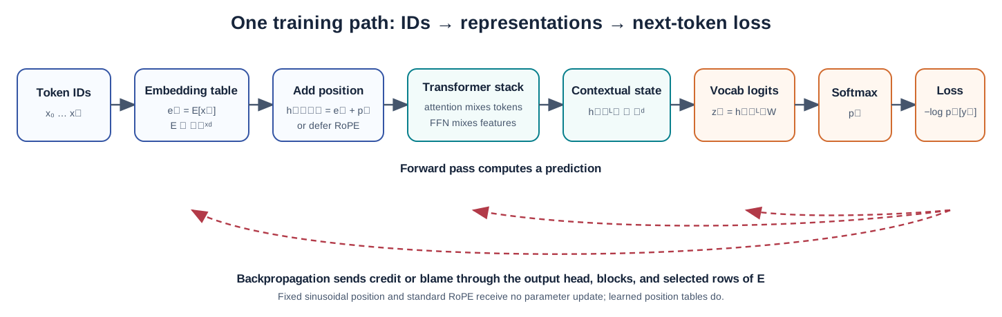
The target coordinate receives a negative correction when its probability is too small; other coordinates receive positive corrections in proportion to their predicted probabilities. Backpropagation carries this signal through the output projection, every Transformer block, the position-combination step, and finally the embedding lookup:

\[ \frac{\partial\mathcal L}{\partial z_t} \longrightarrow \frac{\partial\mathcal L}{\partial h_t^{(L)}} \longrightarrow\cdots\longrightarrow \frac{\partial\mathcal L}{\partial h_t^{(0)}} \longrightarrow \frac{\partial\mathcal L}{\partial E[x_t,:]}. \]

Because lookup selects rows, the input-side gradient for vocabulary row \(v\) is a scatter-add over every occurrence of that ID:

\[ \frac{\partial\mathcal L}{\partial E[v,:]} =\sum_{t:x_t=v}\frac{\partial\mathcal L}{\partial e_t}. \]

If the same token appears five times, those five contributions accumulate in the same row. Rows not selected on the input side receive no input-lookup gradient in that batch. With tied input/output weights, \(E\) also receives an output-side gradient because every row participates in vocabulary scoring.

An optimizer then updates the parameters. A plain gradient-descent step would be

\[ E\leftarrow E-\eta\frac{\partial\mathcal L}{\partial E}, \]

with learning rate \(\eta\). The same loss also updates attention projections, FFN matrices, normalization parameters, and the output head. A learned additive position table receives gradients; fixed sinusoidal encoding and standard RoPE have no positional parameters to update.

12.9 What the whole learning loop accomplishes

The end-to-end chain is

\[ \text{token IDs} \rightarrow E[x] \rightarrow \text{position-aware states} \rightarrow \text{attention and FFNs} \rightarrow \text{contextual states} \rightarrow \text{vocabulary logits} \rightarrow \text{prediction loss}. \]

Backpropagation traverses the same computation in reverse and assigns credit or blame to every learned component. The embedding table learns useful starting coordinates; attention learns how to collect context; FFNs learn feature transformations; and the output head learns how final states support token predictions.

This exposes the two missing pieces that lead into the next chapters:

1. A static embedding does not encode order, so Part 2 adds or injects position.
2. A static embedding cannot choose the context-specific sense of a token, so Part 3 uses attention to create contextual states.

13. Key takeaway

A language model is a system that learns a probability distribution over sequences.

Before it can do that, it must first solve a representation problem:

How do we encode language so that a machine can compare, compress, and reason about meaning?

This leads us through a chain of ideas:

• one-hot: identity only
• counts: statistics
• TF-IDF: weighted statistics
• SVD: latent semantic compression
• Word2Vec: context-based embeddings
• LSTM/RNN: sequential state
• transformer: attention-based context routing

The important idea is simple and deep:

Language modeling is not only about prediction. It begins with building a useful geometry for language.

Without representation, there is no meaning. Without sequence modeling, there is no order. Without attention, there is no rich context flow.

That is the foundation of modern LLMs.

14. The next chapter

The next step is to ask:

How do we preserve sequence order inside a model that no longer depends on recurrence?

That leads us directly into positional encoding and RoPE.